지난 시간에 회귀분석에 대해 간단히 설명드렸습니다. 오늘은 파이썬에서의 실제 구현 과정을 설명하겠습니다. 회귀분석이 기억나지 않는다면 다음 글을 잠시 읽어보세요!
03/17/2023 – (기술/AI, ML, 데이터) – 회귀 분석
회귀 분석
지난번 박스플롯을 이용하여 데이터의 분포를 시각화 했다면 오늘은 회귀분석의 정의에 대해 설명하겠습니다. 제 블로그는 단순한 설명을 넘어 실제 구현까지 다룹니다.
hero-space.tistory.com
데이터
데이터는 이전에 boxplot에 기록된 것과 동일합니다. boxflow는 개별 요인에 대한 데이터의 타당성을 확인하는 것인데, 일정 범위 내에 있었기 때문에 일정 범위 밖의 값에 대한 이상치 측면에서 의미가 있었고, 그것은 데이터 분석 결과가 아니었습니다. 나는 원했다.
앞에서 설명했듯이 데이터 분석에는 두 가지 주요 목적이 있다고 생각합니다.
- 많은 양의 데이터를 분석하려면
- 데이터 간의 상관 관계 또는 통찰력을 얻으려면
그렇기 때문에 작은 데이터로도 엑셀에서 피벗 테이블을 실행해보면 충분히 알 수 있다. 따라서 특정 데이터를 가공하고 분석하는 것은 불필요해 보일 수 있지만 데이터가 쌓일수록 분석이 명확해지고 신뢰도가 높아지므로 이러한 데이터를 Excel이나 수작업으로 분석하는 것은 한계에 도달할 수 있습니다.
데이터 코어
- 자러 갈 시간
- 총 수면 시간(취침 시간 ~ 기상 및 침대에서 일어나는 시간) – 분으로 환산
- 실제 수면 시간(잠드는 시간 – 잠드는 시간 ~ 일어나는 시간) – 분으로 환산
- 일어난 시간
- 중간 휴식 횟수
- 중간에 왜 일어났지?
- 수면의 질에 대한 주관적 평가
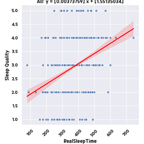
다시, 분석할 요인은 다음과 같다. 이 중에서 실제 수면시간과 주관적인 수면의 질 평가를 X축과 Y축에 구현하여 어떤 결과가 나오는지 확인해 보도록 하겠습니다.
화신
def simple_linear_regression(log, org_data, criteria, without_outliers=False):
    log.info("Simple Linear Regression Start.")
    font_files = font_manager.findSystemFonts(
        fontpaths="./data/font", fontext="ttf")
    for font_file in font_files:
        font_manager.fontManager.addfont(font_file)
    font_name = font_manager.FontProperties(fname=font_files(0)).get_name()
    plt.rc('font', family=font_name)
    plt.rc('axes', unicode_minus=False)

    linear_regression = LinearRegression()

    data = deepcopy(org_data)

    avg_coef = 0
    users = ()
    for user in data.index:
        if user not in users:
            users.append(user)
        else:
            continue

        item_1 = REALSLEEPTIME_MM
        item_2 = SLEEPQUALITY
        log.info("Current Criteria: <" + item_1 + " | " + item_2 + ">")
        x = data(item_1)(user).values.reshape(-1, 1)
        y = data(item_2)(user).values.reshape(-1, 1)

        sns.set(rc={'figure.figsize': (30, 10)})
        plt.rc('font', family=font_name)
        plt.rc('axes', unicode_minus=False)

        linear_regression.fit(x, y)
        print(str(user)+": "+"y = {} x + {}".format(
            linear_regression.coef_(0), linear_regression.intercept_))
        avg_coef += linear_regression.coef_(0)(0)

        curr_at="simple_linear_regression_plus"
        username = user

        output_filename = username+'/'+curr_at+'/'+'random_' + \
            item_1+'-'+item_2+'_regression'+'_simple_linear_plus'

        # check for directory
        if not os.path.isdir(os.getcwd()+'/output/'+username):
            os.mkdir(os.getcwd()+'/output/'+username)
        if not os.path.isdir(os.getcwd()+'/output/'+username+'/'+curr_at):
            os.mkdir(os.getcwd()+'/output/'+username+'/'+curr_at)

        b0 = linear_regression.intercept_
        b1 = linear_regression.coef_(0)

        x_minmax = np.array((min(x), max(x)))
        y_fit = x_minmax * b1 + b0


        sns.lmplot(x=item_1,
                   y=item_2,
                   data=data.query("index == " + "'" + str(user) + "'"),
                   line_kws={'color': 'red'},
                   scatter_kws={'edgecolor': "white"},
                   x_jitter=0.9,
                   robust=without_outliers,
                   palette="coolwarm",
                   height=20,
                   aspect=60/20)

        plt.title(username+": "+"y = {} x + {}".format(b1, b0))
        plt.xlabel(item_1)
        plt.ylabel(item_2)
        plt.xticks(rotation=45)
        plt.savefig(os.getcwd()+'/output/'+output_filename+'.png')

        plt.clf()
    avg_coef /= len(users)
    print("AVG_COEFFICIENT:", avg_coef)

    # All Users
    item_1 = REALSLEEPTIME_MM
    item_2 = SLEEPQUALITY
    log.info("Current Criteria: <" + item_1 + " | " + item_2 + ">")
    x = data(item_1).values.reshape(-1, 1)
    y = data(item_2).values.reshape(-1, 1)

    sns.set(rc={'figure.figsize': (20, 10)})
    plt.rc('font', family=font_name)
    plt.rc('axes', unicode_minus=False)

    linear_regression.fit(x, y)
    print(str(user)+": " +
          "y = {} x + {}".format(linear_regression.coef_(0), linear_regression.intercept_))

    curr_at="simple_linear_regression_plus"
    username="All"

    output_filename = username+'/'+curr_at+'/'+'random_' + \
        item_1+'-'+item_2+'_regression'+'_simple_linear_plus'

    # check for directory
    if not os.path.isdir(os.getcwd()+'/output/'+username):
        os.mkdir(os.getcwd()+'/output/'+username)
    if not os.path.isdir(os.getcwd()+'/output/'+username+'/'+curr_at):
        os.mkdir(os.getcwd()+'/output/'+username+'/'+curr_at)

    b0 = linear_regression.intercept_
    b1 = linear_regression.coef_(0)

    x_minmax = np.array((min(x), max(x)))
    y_fit = x_minmax * b1 + b0

    sns.lmplot(x=item_1,
               y=item_2,
               data=data,
               line_kws={'color': 'red'},
               scatter_kws={'edgecolor': "white"},
               x_jitter=0.9,
               robust=without_outliers,
               palette="coolwarm")

    plt.title(username+": "+"y = {} x + {}".format(b1, b0))
    plt.xlabel(item_1)
    plt.ylabel(item_2)
    plt.xticks(rotation=45)
    plt.savefig(os.getcwd()+'/output/'+output_filename+'.png')

    plt.clf()

    relationship_sleep = data.copy()((item_1, item_2))
    relationship_sleep.to_csv(os.getcwd()+'/output/'+output_filename+'.csv')

    return
scikit-learn 패키지에서는 Linear_regression을 사용하는 것을 제외하고는 그래프를 그려서 이미지로 저장하고 마지막에 원시 데이터를 CSV로 추출합니다. 결과를 보면 다음과 같습니다. 실제 수면 시간(분)이 높을수록 수면의 질이 높아지는 관계는 양의 기울기를 나타냅니다. 물론 그렇지 않은 분들도 계시겠지만, 모든 매개변수에 대한 분석이 이루어졌기 때문에 대체자료 분석이 가능했고, 두 요인이 상당히 높은 상관관계를 가지고 있음을 확인할 수 있었습니다.
그런 다음 주관적인 수면 점수와 잠들기까지 걸린 시간을 비교해 봅시다. 코드에서는 Item1의 요소만 변경하고 다시 실행합니다.
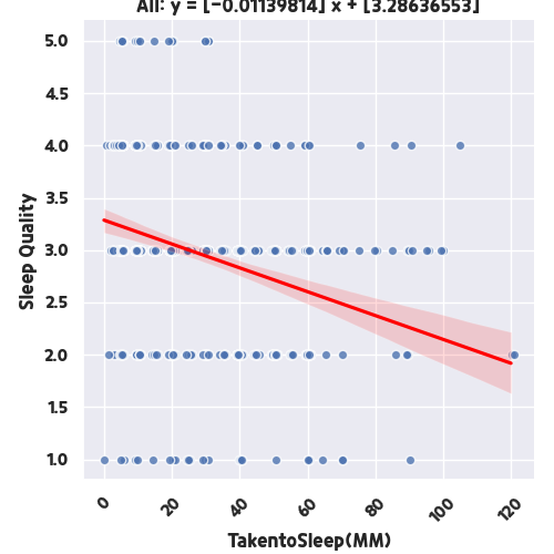
데이터 분석에 따르면 잠드는 데 걸리는 시간이 짧을수록 수면의 질이 좋아집니다. 상식적인 결과지만 데이터 통계나 머신러닝 자체를 이용하는 것보다 데이터 분석이 낫다.
- 데이터를 분석할 수 있도록 처리
- 그것을 시각화하기 위해 다이어그램을 그립니다.
- 지식을 얻는 과정
다음과 같이 정의할 수 있습니다. 마지막 boxplot과 비교하면 어떻습니까? 요인별 상관관계를 볼 수 있으니 이제 다음 단계로 넘어갈 수 있을 것 같습니다. 그런 단위 분석 방법이 꽤 있고, 새로운 것도 많고, 발전함에 따라 최신 트렌드와 기술을 확인하는 습관을 들이는 것이 중요한 것 같습니다. 위의 코드 설명을 자세히 설명하지 않은 이유는 이 코드만으로는 자신의 데이터를 분석하기가 현실적으로 어렵기 때문입니다. 먼저 데이터 분석을 통해 무엇을 하려는지, 어떤 흐름으로 분석해야 하는지 감을 잡을 수 있도록 내용을 공유해드리겠습니다. 다음 데이터 분석 수업에서 만나요!